Mixing Two Cryo-EM Datasets on Purpose: A Cryo-EM Heterogeneity Challenge

Heterogeneity in cryo-EM is both a constant challenge and at the same time one of the technique’s greatest strengths. Biological insights lie within this heterogeneity, in discrete conformational states or continuous structural motions that reveal the functioning of the machinery of life. Yet even experienced cryo-EM scientists can feel as though they are improvising when deciding how best to separate, classify and interpret heterogeneity.

In the Case study: Discrete and Continuous Heterogeneity in FaNaC1 we took a practical approach to this challenge. We combined two publicly available datasets, EMPIAR 11631 (apo FaNaC1) and 11632 (FMRFa-bound FaNaC1), and systematically evaluated different processing strategies to determine which best separates the two particle populations. FaNaC1 is an FMRFa-gated that opens when it binds FMRFa.

Did we manage to recover the FaNaC1 structural states from the mixed dataset?

Tackling Discrete Heterogeneity

This case study explores both discrete and continuous heterogeneity. We begin with discrete heterogeneity, where the goal is to separate the particles from the combined dataset into two well-defined structural states: apo FaNaC1 and FMRFa-bound FaNaC1. To do so, we assume that each particle image is a projection of one of these two rigid volumes in some pose.

3D Classification: to Update the Poses, or Not to Update the Poses?

The first strategy we tested for separating the apo and FMRF-a bound FaNaC1 states was 3D Classification into two classes. Starting from a high-resolution consensus refinement generated from the mixed particle stack, we applied a solvent mask to the whole protein volume and a focus mask to the extracellular domain, which contains the FMRFa binding site and undergoes the largest conformational changes upon ligand binding.

Because the consensus refinement had already converged to high resolution, we did not update the particle poses throughout classification. The Heterogeneous Reconstruction Only of the two resulting classes revealed something interesting: although the particles separated into an apo-like closed state and an FMRFa-bound open state, closer inspection of the apo-like map showed residual density in the FMRFa binding site.

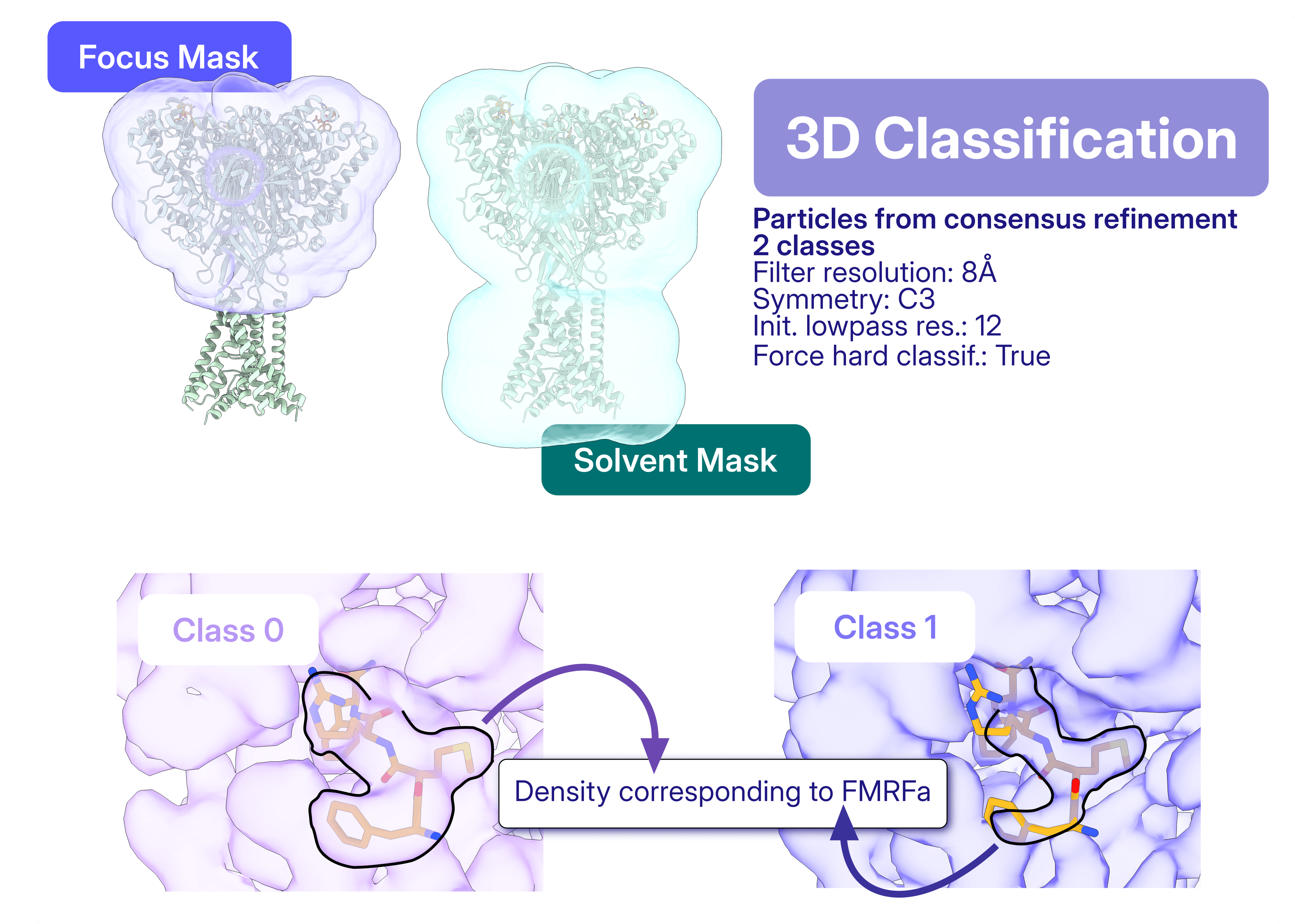
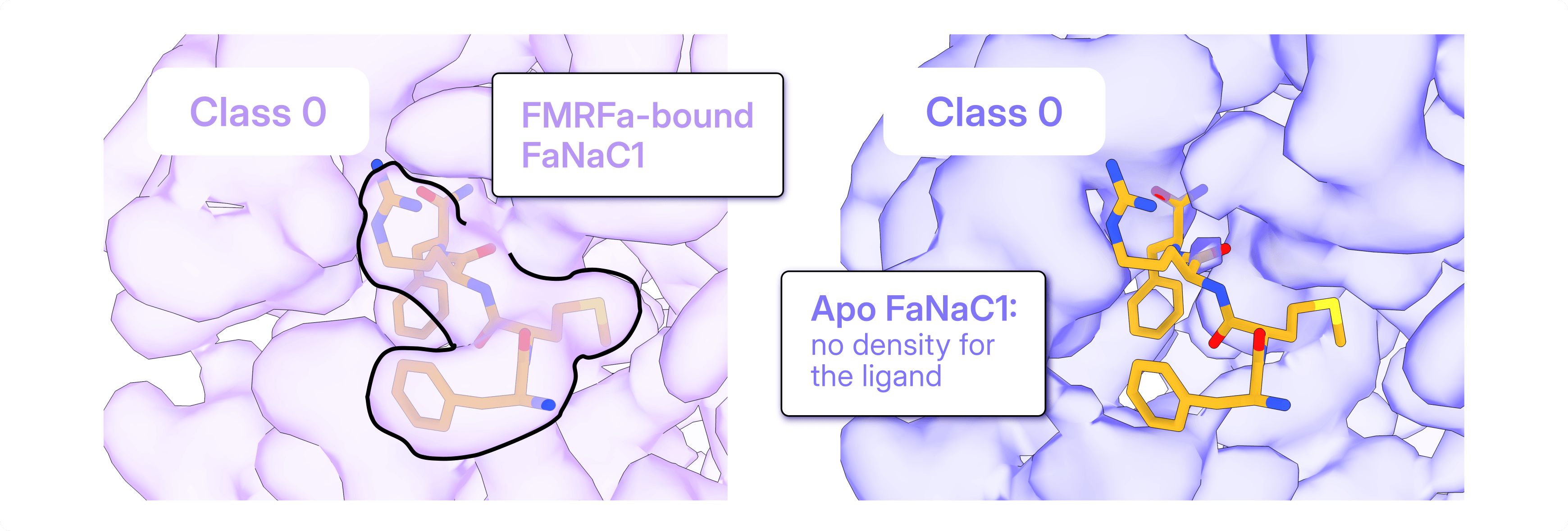
FRMFa-bound AND closed? Since FaNaC1 is known to open rapidly upon FMRFa binding, this result raised important questions. Was the 3D classification contradicting the expected biochemical behavior, and there is indeed partial occupancy of FMRFa in the apo structure? Had it failed to separate the two FaNaC1 states? Or was the apparent ligand density a consequence of keeping particle poses fixed during 3D Classification?

The apo structure also contained blurry, smeared-out regions of density, which could reflect residual heterogeneity, local flexibility, or imperfect particle alignment. To test this, we re-refined the particles from each class separately using Non-Uniform Refinement, updating the particle poses within each subset. The resulting maps were consistent with the original class reconstructions, confirming that 3D Classification had successfully separated the particles into closed and open states. However, after separate pose refinement, the apo-like closed map no longer showed FMRFa density in the binding site. This indicated that FMRFa was bound only in the open FaNaC1 state, and that the apparent ligand density in the closed class arose from the limitations of reconstructing each class with fixed poses.

Heterogeneous Refinement: Classification and Pose Refinement Together

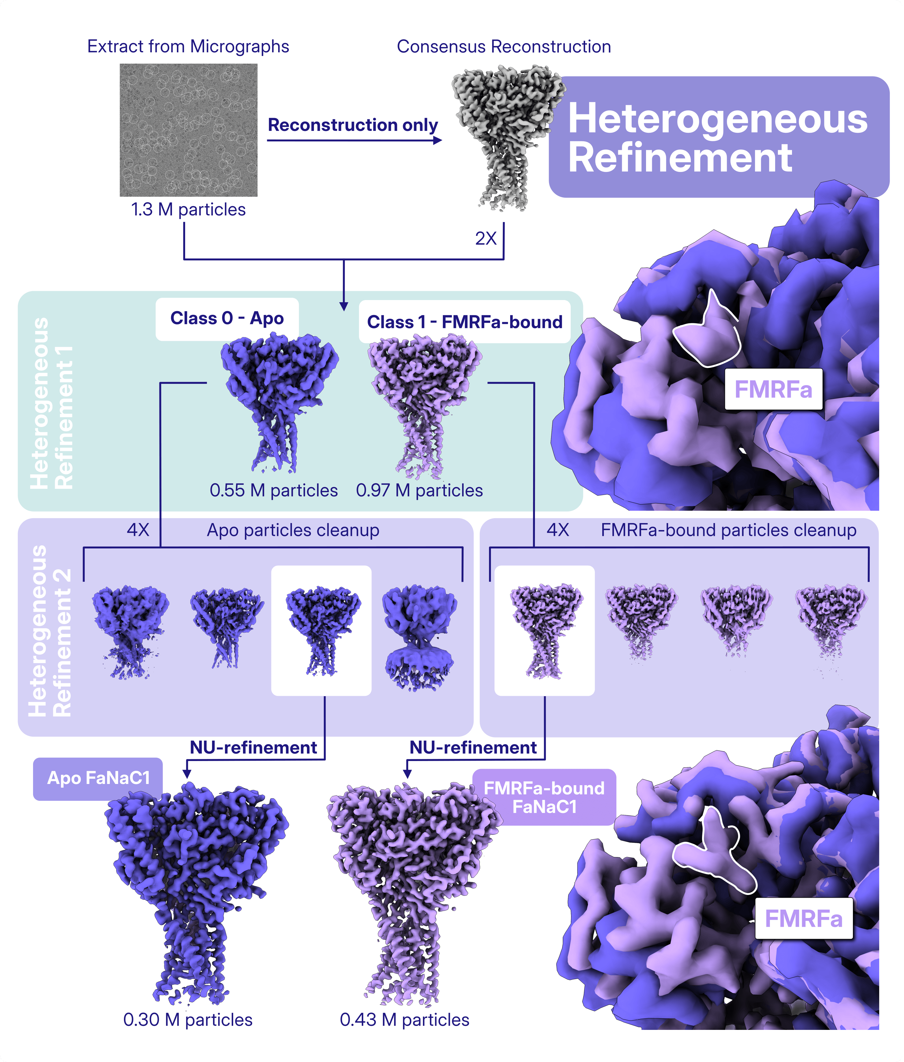
The second approach was Heterogeneous Refinement, which performs classification and pose refinement simultaneously. As in the previous strategy, we set up the job with two identical copies of the consensus map. Starting from the mixed particle stack, Heterogeneous Refinement successfully separates apo and FMRFa-bound conformations, while refining the particle alignments for each class.

However, the apo reconstruction presented lower map quality when compared to the FMRFa-bound structure, hinting at the possibility of the presence of junk particles in the apo particle stack. Heterogeneous Refinement can also be used as particle-cleanup step, and to filter out these junk particles it was enough to:

• separately refine apo and FMRFa-bound particles, and
• increase the copies of the respective volumes as inputs for the Heterogeneous Refinement job.

By refining each particle stack against four identical copies of its respective reference volume, one class consistently emerged as the highest-quality reconstruction. This class converged to the respective FaNaC1 state, while the remaining classes captured lower-quality, poorly aligned, or otherwise less consistent particles.

Exploring Continuous Heterogeneity

In reality, proteins do not simply snap from one conformation to another, rather they exist on a continuum of structural states, forming a conformational landscape. Discrete classification approximates this landscape by dividing it into a finite number of structural states and assigning each particle to one of them. In contrast, continuous heterogeneity models each particle as originating from a slightly different conformation, represented as a deformation of a consensus structure. How and when do we model continuous heterogeneity?

3D Variability Analysis: Choosing the Right Modes

3D Variability Analysis (3DVA) explores continuous heterogeneity using Principal Component Analysis (PCA), identifying the dominant ways a protein changes shape across a dataset. Rather than assigning particles to a small number of discrete classes, 3DVA describes each particle as a combination of a few common motions.

To obtain meaningful results, the input particles should be as clean and well aligned as possible, and the input mask should encompass the entire region expected to move, since structural changes are only modeled within the masked region. Two parameters largely determine what 3DVA will reveal:

• Number of Modes: how many independent motions the algorithm should identify.
• Filter Resolution: the spatial scale of the motions that will be modeled. Higher filter resolutions allow finer structural changes to be captured.

Choosing these parameters is often an iterative process, as there is no way to know the optimal settings beforehand. In this example, we explored both 1 and 2 Modes to determine whether the conformational changes associated with FMRFa binding are best described as one concerted motion or two independent motions. The Filter Resolution was set to 4 Å, based on the structural differences observed during the discrete heterogeneity analysis.

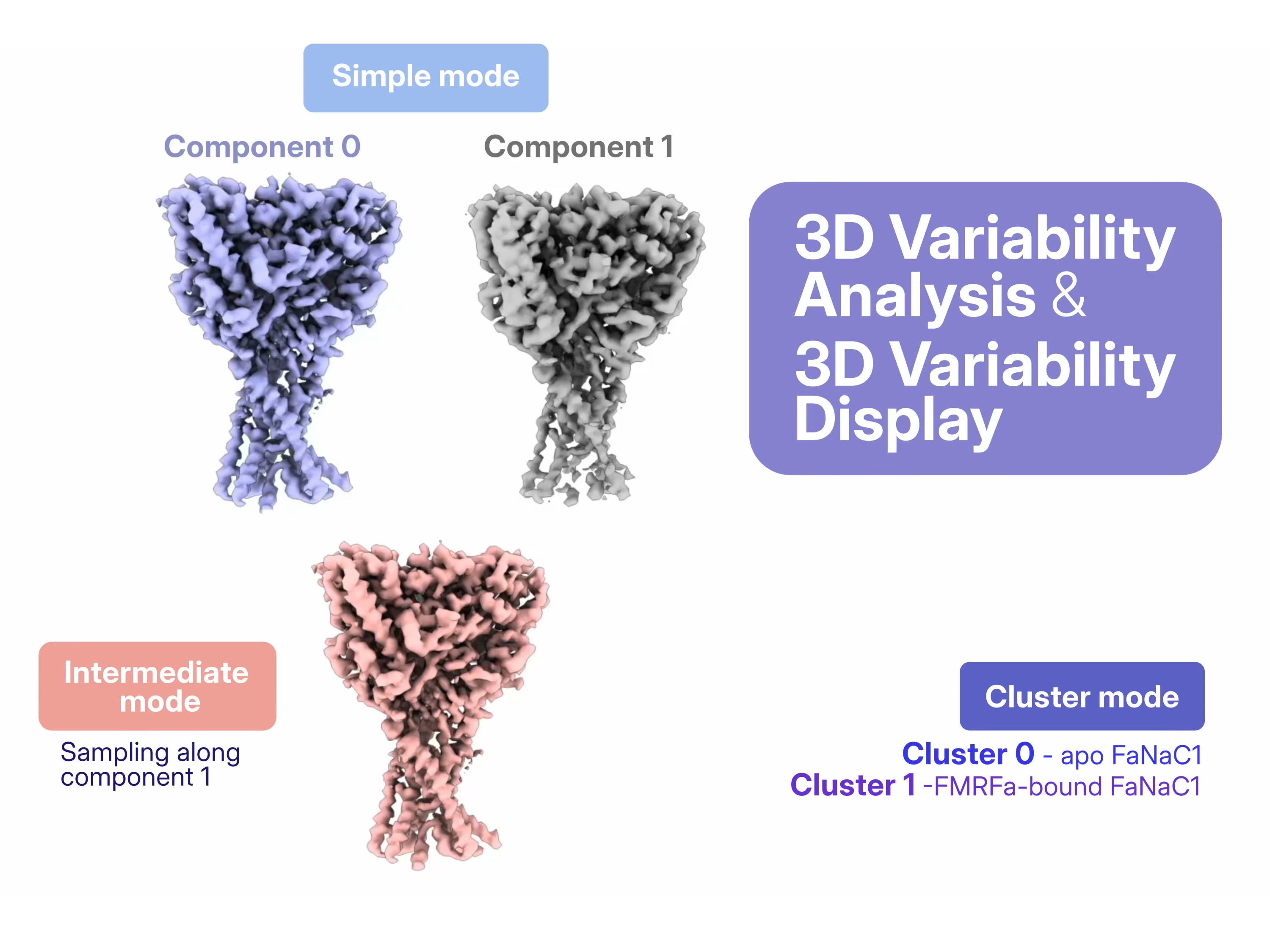
While 3DVA computes the variability model and produces useful diagnostic plots, 3D Variability Display is used to visualize it. It offers three complementary visualization modes:

• Simple Mode: generates synthetic maps by adding or subtracting variability components from the consensus reconstruction. This makes it easy to inspect the effect of each component individually.
• Intermediate Mode: groups particles along a selected variability component and reconstructs maps from the original particle images, producing more realistic reconstructions.
• Cluster Mode: clusters particles using all variability components simultaneously and reconstructs one map per cluster, making it particularly useful for recovering distinct structural states.

In 3D Variability Display, the Filter Resolution determines the resolution at which the output volumes are reconstructed and visualized.

Using two Modes (or components) in 3DVA, Simple Mode revealed two dominant motions. The first captured the expected conformational changes associated with FMRFa binding, while the second highlighted motion within the transmembrane domain. Whether this second motion is biologically meaningful or represents a separate source of variability is not immediately obvious, illustrating why interpreting individual components often requires additional context.

Using the component corresponding to the expected conformational changes upon FMRFa binding in Intermediate Mode produced higher-quality maps. Because these reconstructions are generated from the original particle images rather than synthetic combinations of variability components, they retain the contributions of the remaining motions and provide a more faithful representation of the underlying conformational landscape.

Finally, Cluster Mode (using two clusters) cleanly separated the apo and FMRFa-bound particle populations. The resulting reconstructions can be refined further, making Cluster Mode a practical bridge between continuous heterogeneity analysis and conventional high-resolution refinement.

3D Flexible Refinement: Are There Enough Particles in Intermediate States?

While 3D Variability Analysis models conformational changes as combinations of linear motions, 3D Flexible Refinement (3D Flex) takes a different approach: it models deformation and movement of a tetrahedral mesh around the consensus volume. The deformation of the generated mesh rather than the volume voxels reduces the degrees of freedom, preventing unrealistic motions and overfitting.

Compared with the previous methods, 3D Flex requires additional preparation steps, including particle cropping and downsampling, mask and mesh generation, and iterative rounds of 3D Flex Train and 3D Flex Generate. The main challenge in this case study was tuning the 3D Flex Train parameters. In particular, rigidity and latent centering strength had a profound effect on the modeled motions and required several rounds of optimization. 3D Flex Generate was then used after each training round to inspect the learned conformational landscape and guide the next set of parameters.

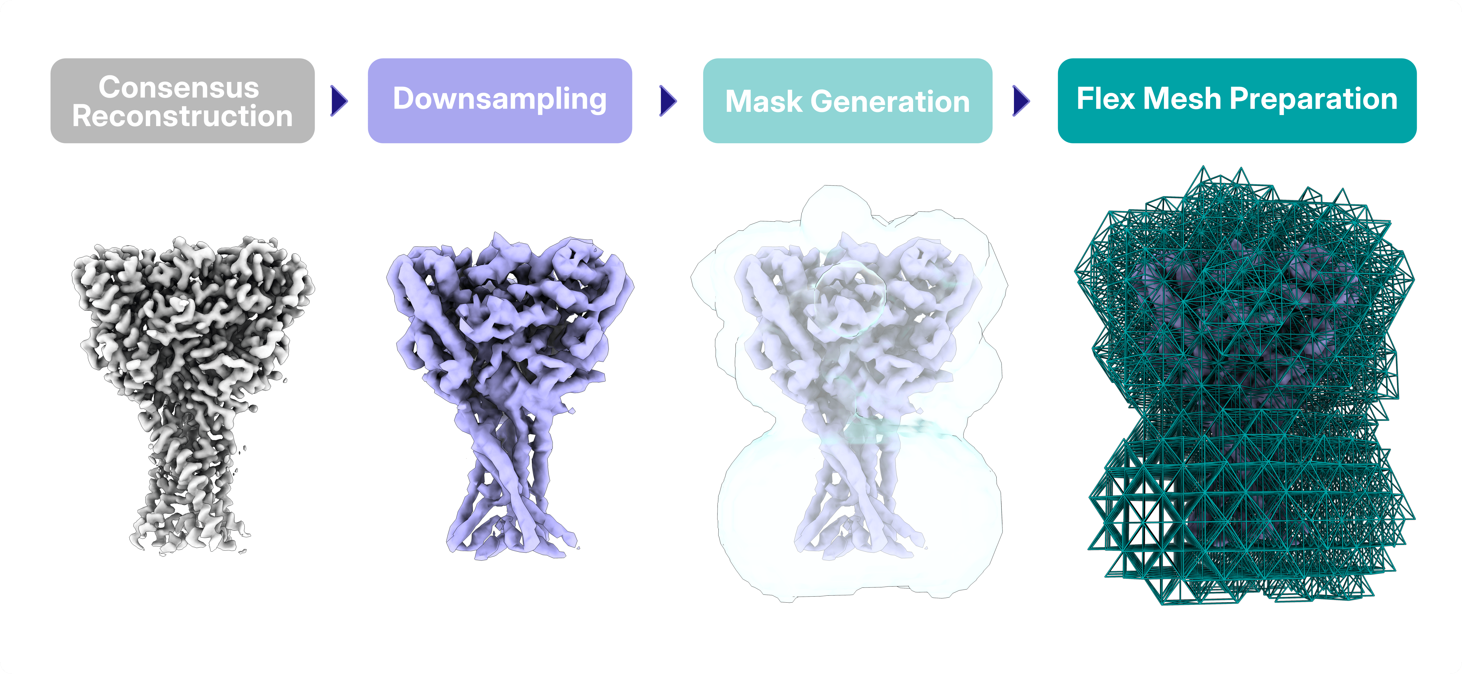
In this FaNaC1 example, the first training runs produced only limited conformational changes. By iteratively reducing the rigidity and latent centering strength, the latent space expanded and the expected movement of the FaNaC1 domains gradually emerged, consistent with the motions observed by 3D Variability Analysis. However, lowering these parameters too far introduced unrealistic "jelly-like" deformations of the transmembrane helices, illustrating the balance between capturing realistic flexibility and avoiding non-physical motion.

When and How to Look for Heterogeneity

This deliberately mixed dataset provides an excellent opportunity to understand how different heterogeneity analysis methods behave, how their parameters influence the resulting maps and motions, and how to assess whether the conformational changes revealed by 3D Variability Analysis and 3D Flexible Refinement are physically meaningful.

The biology of the sample should guide the interpretation of every result and users should continually ask whether the observed structures make biological sense. Is FMRFa really bound to the closed conformation? Could the map improve by further cleaning or classifying the particles? Are the observed motions concerted or independent? Are there enough particles sampling intermediate conformations to justify modelling continuous heterogeneity?

There is no universally "best" approach to heterogeneity analysis. The appropriate workflow depends on both the sample and the biological question being asked. By comparing 3D Classification, Heterogeneous Refinement, 3D Variability Analysis, and 3D Flexible Refinement on the same dataset, this case study illustrates the strengths, limitations, and practical considerations of each method, providing a roadmap for choosing the right strategy for your own cryo-EM data.